Backtracking algorithms: experiment, inspect and adapt

In this article I tell the story of a beautiful picture which represents an interesting mathematical problem whose algorithmic solution has some analogy to the agile way of solving problems and making progress.

The picture

My former high school math teacher Hansruedi Widmer (“retired as a teacher, not as a mathematician”) daily posts mathematical puzzles, bits of history or just “fun facts” on X (formerly known as twitter). Two years ago, on March 1^st, 2022, which was the 60^th day of the year, he tweeted the following (translation from German is mine):

As it is day 60: The numbers from 1 to 60 can be paired in such a way that the sum of every pair is one of the square numbers 3², 6², 7², 8², 9².

— tweet by Hansruedi Widmer on March 1^st, 2022

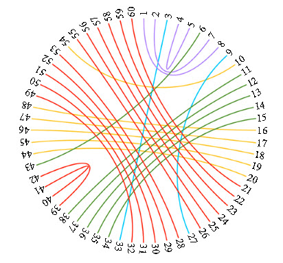
I found (and still find) this drawing (figure 1) very beautiful, like a piece of art, and I wanted to know more about the underlying mathematical problem:

1. Is there more than one solution which satisfies the given constraints?
2. And if yes, how can they be found?

I have been thinking, experimenting and writing about this problem every once in a while, time and again, but something (new job, continuing professional education, family) always got in the way of finishing this article. But finally, on the occasion of the 60^th day of this year - which, because it is a leap year, is not on March 1^st but on February 29^th - I got it done. I hope you enjoy reading it as much as I enjoyed writing it.

The problem

I asked Hansruedi, but all he could tell me without further investigation was that 93 pairs could be formed with the numbers from 1 to 60 whose sum was an element of the set {9, 36, 49, 64, 81}. The solution was to choose 30 out of these 93 pairs such that every number from 1 to 60 was included exactly once.

The 93 pairs can easily be found by iterating over all numbers i from 1 to 60 and checking for every number j between (i + 1) and 60 whether the sum of i and j is an element of the above set of square numbers:

• 1 can be paired with 8 (to yield 9), with 35 (to yield 36) and with 48 (to yield 49)
• 2 can be paired with 7 (to yield 9), with 34 (to yield 36) and with 47 (to yield 49)
• 3 can be paired with 6 (to yield 9), with 33 (to yield 36) and with 46 (to yield 49)
• 4 can be paired with 5 (to yield 9), with 32 (to yield 36), with 45 (to yield 49) and with 60 (to yield 64)
• 5 can be paired with 31 (to yield 36), with 44 (to yield 49) and with 59 (to yield 64)
• and so on

Alternatively, of course, the pairs can be found the inverse way, by iterating over all numbers i from 60 down to 1 and checking for every number j between (i - 1) and 1 whether the sum of i and j is an element of the target set.

A table with all pairs sorted in different ways can be found here.

The difficult part is to find 30 pairs out of these 93 which satisfy the additional constraint that every number from 1 to 60 is included exactly once.

As Hansruedy had not investigated this any further, I had to give it a try myself.

The solution

1^st attempt: a dead end

Maybe pushed a bit into this direction by Hansruedi’s very mathematical problem description (“Choose 30 out of these 93 pairs such that …") I tried exactly that: Somehow generate all possible subsets of 30 pairs out of the whole set of 93 pairs and then apply the additional constraints. None of my experiments worked, and if you look at the sheer dimension of the problem, it becomes obvious that none of them could work, at least not with today’s computers:

Combinatorics tells us that the number of possible ways to choose 30 pairs out of 93 is

“93 choose 30” = 93! / (30! x (93-30)!) = 93! / (30! x 63!)

which is 2.200 x 10²⁴, i.e. 2.2 septillion, which is an enormous number (22 followed by 23 zeroes).

A web search led me to the paper from the Mathematical Association of America( MAA) from which the above picture must have been taken. I learned that the problem is called “rainbow squares” because of the way in which the pairs with equal sum are marked with the same color, or simply “rainbow pairs” for the more general case where the sums are subject to some constraint different from being square numbers (e.g. polynomials or Fibonacci numbers).

I also learned from this paper that the number of solutions for the numbers from 1 to 60 where the sum is constraint to be any square, i.e. {4, 9, 16, 25, 36, 49, 64, 81, 100} is 4,366,714! But how many solutions would there be with the narrower constraint set {9, 36, 49, 64, 81}? And how could they be found?

2^nd attempt: slowly getting there

As the purely mathematical approach had not worked, I tried to think about the problem more procedurally: Not in terms of selecting pairs but in terms of drawing the beautful picture shown in figure 1: If I had a sheet of paper with the circle of numbers from 1 to 60 and five colored pencils, how would I go about drawing such a picture?

Starting with the empty “circle” (figure 2):

I would begin with the lowest number - 1 - and tentatively mark a pair for it. I could use any of the three possible pairs shown in the reference table, so to do it sistematically, I would just choose the first one from the second column in the table. This is the lowest pairing, which is 8 (figure 3):

I would do the same for the next three numbers 2 to 4 (figure 4):

As the numbers 5 to 8 are already paired, I would continue with 9 to 17 (figure 5):

And 18 (figure 6):

Again, as the numbers 19 to 27 are already paired, I would continue with 28 to 30 (figure 7):

And then all the numbers from 32 to 40 which have not already been paired (figure 8):

And as numbers 41 to 44 have already been paired, I would now like to continue wth 45, but there is a problem: As can be seen in the reference table, there is no more pairing possible for 45. What to do now?

As I have said at the beginning, I have just marked the pairs tentatively, so I can now trace back and erase the latest pair marked ([40 - 41]) (figure 9):

Unfortunately, this is not enough because at this point I have no alternative for number 40 than to pair it with 41. So I have to trace further back until I arrive at the number for which there is an alternative path forward. This is number 30 (figure 10):

Instead of pairing 30 with 34, I now pair it with 51 (figure 11):

And continue forward from there until I run into another dead end, which happens to be at number 45 again (figure 12):

So I have to trace back to 30 again, but as there is no third alternative besides 34 and 51 for 30, I have to trace yet another step back to 29 and pair it with 52 instead of 35 (figure 13):

And from here I can move forward again. And back and forth and back and forth again… And if there is a solution, I will eventually find it. But how long will it take?

Millions of repetions of the same small, simple step? Sounds like the perfect problem to write a program for!

This type of algorithm is called backtracking algorithm as I remembered from the time I had once implemented a Sudoku solver in Ruby some 20 years earlier. Sudoku is a very typical application of backtracking, as is the Eight Queens Problem with which the algorithm is usually illustrated in textbooks. But the rainbow squares problem is equally well suited to illustrate backtracking, as I hope to have shown above.

I implemented the algorithm in python. The program file can be found here and its output file here. I will not explain the program here; I will explain the final version at the end of this solution section.

This first version worked exactly as shown in the figures above. It found 5294 solutions but ran 48 minutes on my machine (normal laptop, not quite new, nothing optimized, so the measurement is just for relative comparison with the improvements shown further below). That was disappointing and unexpected, because for an average Sudoku, a backtracking algorithm finds the solutions in a few seconds or even less than a second. Analysis showed that the algorithm had performed 5.2 billion tentative steps whereas an average Sudoku only requires something between 10,000 and 100,000 or in an extreme case maybe a million steps. The reason is that Sudokus are very highly constraint puzzles where many alternatives can be excluded early on. For this problem, on the other hand, even the first solution is only found after more than 47 million steps which means I could never have found it by hand within my lifetime.

3^rd attempt: backward is faster

How could the algorithm for the rainbow squares be improved? I found a hint in the AMM paper mentioned above where for a simpler problem (numbers only from 1 to 18, not to 60) they ask whether it would be better to start with small pairs or large ones and answer that “The latter is in fact more efficient since it presents fewer choices early on.” That the same holds for our problem with numbers from 1 to 60 can be seen in the reference table: While the twelve smallest numbers can form three or even four pairs each, the twelve largest numbers can only form two pairs each.

I changed the algorithm to run backwards from 60 to 1. Again, the program file can be found here and its output file here. And again, I will not explain the program here; I will explain the final version at the end of this solution section.

Running backwards reduced the number of tentative steps from 5.2 billion to 112 million and the execution time on the same machine from 48 to 2 minutes! And the first soluton is found after only 61 steps. This could be done by hand.

Why does the direction in which the algorithm runs have such a massive effect? The answer is that conceptually, the algorithm searches a tree of possibilities. Running it from 60 to 1 instead of from 1 to 60 changes the structure of this tree (figure 14):

Starting with the largest pairs yields a tree which is narrower but deeper as - with a bit of imagination - could already have been seen in the reference table. Or as the AMM paper states: “… it presents fewer choices early on.”

Another strategy which might be worth exploring is to run from 1 to 60 but for each number start with the highest-number pairing instead of the lowest one, i.e. pair 1 first with 48, 2 with 47, 3 with 46, 4 with 60 and so on. Thinking in terms of the tree, this means leaving the structure of the tree unchanged but exploring different branches first. I have not tried this.

I was not so interested in exploring these kinds of optimization any further because they are highly dependant on the concrete problem. Does the statement “… it presents fewer choices early on…” still hold if the target set is not a set of square numbers but e.g. of prime numbers? This would have to be analyzed for every case separately.

4^th and final attempt: fast forward

The generic algorithm might benefit from tree optimization techniques, either up-front before starting the traversal, or even at every step of the search. But I have no experience with such techniques and have not explored them any further.

Besides the two optimization techniques just mentioned (optimizing the tree and optimizing the order in which the subtrees are searched at any given node), there is only one more area for optimization: making sure that all possible information is taken into account at every step to decide whether to continue the search in this direction or not.

Looking at my paper figures again and thinking a bit more about the forward and backward running algorithms, I suddenly found the missing piece: In the first version of my algorithm, on the first traversal “down the tree”, I chose the 11^th pair to be [15 - 21] as shown in figure 5 because that’s the first option listed for 15 in the second column of the reference table and because the number 21 is not yet used by any other pair which means it is still available (figure 15):

But taking also the fourth column of the table into account (for all numbers greater than 15), I see that 60 can only be paired with 4 and 21. As 4 is already paired with 5, I cannot pair 15 with 21 now; I have to leave 21 free to be paired with 60. I will therefore try the second option for 15 right away, which is 34. I thus save myself from taking a wrong turn at this junction and traversing many additional subtrees which would not yield any result. 16 on the other hand can be paired with 20 as in the initial version of the algorithm (figure 16):

Taking this effect of the current pairing on potential future pairings into account allows to stop and retrace much earlier, i.e. cut off huge subtrees of the search tree which otherwise would have been traversed without any result.

If this additional check is incorporated into the forward-running algorithm which before took almost an hour to run and executed 5.2 billion steps, the program reaches roughly the same execution time as the backward-running algorithm (around 2 minutes) and uses less than 2 million steps! The number of steps is massively smaller even than for the backward-running algorithm (which needs 112 million steps) but unfortunately there is no further improvement on execution time as more checks have to be performed at every step. Performance-wise, the two effects seem to cancel each other out. Nevertheless, this final version of the algorithm is superior to the backward-running version because the optimization applied is more general, i.e. independent of the concrete problem and its tree structure. It will generally perform better also for other target sets like Fibonacci numbers or prime numbers. Of course, the different optimization strategies could all be combined, but as explained above, I had no interest in analysing specific optimizations for specific trees any further.

As promised, I will now show and explain the full program in its final version:

  1import functools
  2
  3# function which calculates and returns the set of all possible pairs of numbers
  4# from 1...N which satisfy the condition that their sum is in the targets set
  5def possible_pairings(N, targets):
  6  result_list = []
  7  for i in range(1, N+1):
  8    result_list.append([])
  9  for i in range(1, N+1):
 10    for j in range(1, N+1):
 11      if i != j and i + j in targets:
 12        result_list[i-1].append(j)
 13  return result_list
 14
 15# global counter to keep track of the number of solutions found
 16solution_count = 0
 17
 18# global counter to keep track of the number of recursive solver calls
 19recursion_count = 0
 20
 21# recursive solver procedure
 22def solve(pos):
 23
 24  global recursion_count
 25  recursion_count = recursion_count + 1
 26
 27  # if all positions in the circle have been taken,
 28  # a solution to the puzzle has been found
 29  if pos == N+1:
 30    global solution_count
 31    solution_count = solution_count + 1
 32    log = "After " + str(recursion_count) + " total calls to 'solve()': "
 33    log = log + "solution no " + str(solution_count) + ": "
 34    print(log)
 35    print(used_pairs)
 36
 37  # if the current position in the circle has already been taken by the second
 38  # element of a pair placed earlier, then move on to the next position
 39  elif pos_taken[pos-1]:
 40    solve(pos+1)
 41  else:
 42
 43    # else iterate over all possible pairs for the current position
 44    for paired_pos in possible_pairs[pos-1]:
 45
 46      # if the position of the pair's second element is also available...
 47      if not pos_taken[paired_pos-1]:
 48
 49        # ... then remember the currently used pair
 50        # and tentatively mark both positions in the circle.
 51        used_pairs.append([pos, paired_pos])
 52        pos_taken[pos-1] = True
 53        pos_taken[paired_pos-1] = True
 54
 55        # The above three lines already simulate the current move; 
 56        # check its effects before actually making the move 
 57        # and stepping one level down the tree.
 58
 59        # positive assumption: all future pairs reachable, i.e. for
 60        # every position not yet taken, there exists a pair position
 61        # not yet taken
 62        all_future_pos_reachable = True
 63
 64        # for every future position, try to prove assumption wrong 
 65        for p in range(pos+1, N+1):
 66          if not pos_taken[p-1]:
 67                      
 68            # negative assumption: no more pair position available
 69            paired_p_reachable = False
 70
 71            # try to prove assumption wrong 
 72            for paired_p in possible_pairs[p-1]:
 73              if not pos_taken[paired_p-1]:
 74                paired_p_reachable = True
 75                
 76            if not paired_p_reachable:
 77              all_future_pos_reachable = False
 78
 79        if all_future_pos_reachable:        
 80          # move on to the next position
 81          solve(pos+1)
 82
 83        # trace back by releasing the used pair 
 84        # and unmarking the two positions in the circle
 85        used_pairs.pop()
 86        pos_taken[pos-1] = False
 87        pos_taken[paired_pos-1] = False
 88
 89# upper bound N of the interval of numbers 1...N in the circle
 90N = 60
 91
 92# set of target numbers for the pairs
 93targets = (9, 36, 49, 64, 81)
 94
 95# the set of possible pairs which satisfy the target 
 96possible_pairs = possible_pairings(N, targets)
 97
 98# list of the positions 1 ... N to keep track of 
 99# which are already taken and which are still unoccupied
100pos_taken = []
101for i in range(1, N+1):
102  pos_taken.append(False)
103
104# list of all the pairs currently used in the backtracking algorithm
105used_pairs = []
106
107log = "Calculating Rainbow Pairs for 1 ... " + str(N)
108log = log + " for target set " + str(targets) + ":"
109print(log)
110print()
111print("Possible partner positions for each position 1 ... " + str(N) + ":")
112print(possible_pairs)
113print()
114
115li = list(map(lambda li: len(li), possible_pairs))
116num_pos_pairs = round(functools.reduce(lambda a, b: a+b, li)/2)
117print("Number of possible pairs: " + str(num_pos_pairs))
118
119solve(1)
120
121print()
122log = "Calculation terminated. " + str(solution_count)
123log = log + " solutions found with " + str(recursion_count)
124log = log + " calls to recursive solver function."
125print(log)

The main program begins on line 89:

• 90: Definition of the interval 1 … N = 60
• 93: Definition of the set of target numbers {9, 36, 49, 64, 81}
• 96: Calculation of the set of possible pairings. The term “set” is actually imprecise here as the solve procedure depends on the data structure exactly as returned by the auxiliary function possible_pairings: a list of N lists where each list corresponds to the possible pairings for number i, i running from 1 to N. This corresponds exactly to the fourth column of the reference table. Because each pair is listed twice, the total number of pairs in our example is 186.
• 98 - 105: The two data structures pos_taken and used_pairs together correspond to my paper drawings: They track the current state of the partial solution:
  • pos_taken keeps track of which positions in the circle are already marked by a pair. The list is initialized with all False values as initially no position is taken.
  • used_pairs keeps track of the pairs used in the current partial solution. This is needed to print the solution when one has been found. The list is initially empty.
• 107 - 117: Some initial output
• 119: Execution of the solve procedure for the first position. As this is a recursive procedure, it will execute again and again until all solutions have been found.
• 121 - 125: Some final output

The main program depends on functions, procedures and variables defined and implemented in lines 1 - 76.

Lines 1 - 19 contain a function implementation and the definition of two counters:

• 5 - 13: Function possible_pairings calculates the list of possible pairings. In the problem section above, I said that the 93 pairs can easily be found by iterating over all numbers i from 1 to 60 and checking for every number j between (i + 1) and 60 whether the sum of i and j is an element of the above set of square numbers. As in the final version of the program we consider forward and backward information, we need all pairs listed twice, once for the lower number and once for the higher number. That’s why j also runs from 1 to 60, not only from (i + 1) to 60.
• 16: Definition of a counter for the number of solutions already found.
• 19: Defintion of the number of recursions already executed, i.e. the number of times procedure solve has already been called.

Lines 21 - 87 contain the definition and implementation of the solve procedure which contains all the backtracking logic:

• 25: Increment the recursion counter
• 29: If we are at position N+1, a solution has been found:
  • 31: Increment the solution counter
  • 32 - 35: Print the current solution
  • Do nothing more in this recursive step. This means: Jump back to the context of the caller of solve(N+1) which in turn is an execuction of solve, namely solve(N).
• 39/40: Else if we are at a positition smaller than N+1 which is already taken (i.e. paired with a lower position), then we move on to the next position, i.e. recursively call solve(pos+1).
• 41: Else (i.e. if we are at a positition smaller than N+1 which is unoccupied):
  • 44: We loop over all possible pair positions of the current position:
    • 47: If a possible pair position is not already taken (i.e. paired with a lower position), then
      • 51 - 53: Tentatively add the current position and the current pair position to the list of used pairs and mark the current position and the possible pair position as taken.
      • 55 - 77: These 23 lines are the main improvement over the initial version of the program, causing the execution time to improve by a factor of 24 and the number of recursive calls to decrease by a factor of more than 2500: Check for all positions not yet taken, whether there also exists a possible pairing not yet taken.
      • 79/81: Only if all future positions are still reachable, keep the current pair and move on to the next position, i.e. call solve(pos+1).
      • 83 - 87: At this point, either solve(pos+1) has been executed (which includes all its recursive executions) because all future position were still reachable with the current pair, or it has not been executed because at least one future position would no longer have been reachable. In the first case, we are now on the way up the tree again and have to undo the current pairing made in lines 51 - 53. In the second case, we could not make the step down the tree and have to undo the (tentative) pairing just the same.

The program file can be found here and its output file here. The output file shows that the final version of the program finds the solutions in the same order as the initial version but just performs a lot less unneccessary steps.

The analogy

I like backtracking algorithms for several reasons. Remember the drawing of the Rainbow Squares Circle which got me started with this article? I do not only find this drawing very beautiful, but also the algorithm which allowed me to find the solutions to this puzzle. I find the concept of backtracking very elegant. I like to watch animations of backtracking algorithms like for example this one for the Eight Queens Puzzle.

Backtracking algorithms in their efficiency also remind me a lot of the agile way of working: experiment, inspect and adapt: try something, measure its effect, and if it does not work, then try something else. But do it systematically and empirically.

The three empirical pillars of scrum are transparency, inspection and adaptation. Transparency and inspection are important here: We have been able to improve the efficiency of the algorithm massively by including information previously ignored. If something does not work, it is crucial to fail at the earliest possible moment and not waste time exploring dead ends any further. As the scrum guide states:

• Transparency enables inspection. Inspection without transparency is misleading and wasteful.
• Inspection enables adaptation. Inspection without adaptation is considered pointless.